Ejercicios#
import numpy as np
Convoluciones de arrays#
Exercise 55
Dadas dos funciones de variable real \(f\) y \(g\), definimos la convolución de \(f\) y \(g\) como
La versión discreta de la anterior definición puede ser la siguiente. Datos \(f=(f_0, \dots, f_{n-1})\) y \(g=(g_0, \dots, g_{m-1})\) dos vectores (representados por arrays unidimensionales) de tamaño \(n\) y \(m\), respectivamente, definimos el array conv de dimensión n + m - 1 cuya componente \(k\) vale
para \(0 \leq k \leq n + m - 1\).
Crea una función conv que tome como inputs dos arrays y devuelva la convolución de ambos. Por ejemplo
arr1 = np.arange(10)
arr2 = np.arange(5)
conv(arr1, arr2)
>>> [ 0  4 11 20 30 40 50 60 70 80 50 26  9  0]
def conv(f, g):
    n = f.size
    m = g.size
    conv = np.zeros(n + m - 1)
    for k in range(n + m - 1):
        terms = []
        for i in range(n):
            for j in range(m):
                if i + m - 1 == k + j:
                    terms.append(f[i]*g[j])
        conv[k] = sum(terms)
    return conv


f = np.arange(10)
g = np.arange(5)
conv(f, g)
array([ 0.,  4., 11., 20., 30., 40., 50., 60., 70., 80., 50., 26.,  9.,
        0.])
def conv(f, g):
  n = f.size
  m = g.size
  convolucion = np.zeros(n + m - 1)
  for k in range(n + m - 1):
      for i in range(max(0, k - m + 1), min(k + 1, n)): # Esto es lo que faltaba
        j = i + m - 1 - k
        convolucion[k] += f[i] * g[j]

  return convolucion

arr1 = np.arange(10)
arr2 = np.arange(5)
print(conv(arr1, arr2))
Procesando imágenes con numpy#
Exercise 56
Una de las posibles técnicas que existen para comprimir una imagen es utilizar la descomposición SVD (Singular Value Decomposition) que nos permite expresar una matrix \(A\) de dimensiones \(n\times m\) como un producto
donde \(U\) y \(V\) son cuadradas de dimensiones \(n\) y \(m\) respectivamente y \(\Sigma\) es diagonal y está formada por los valores singulares de \(A\) ordenados de mayor a menor (siempre son números reales y positivos).
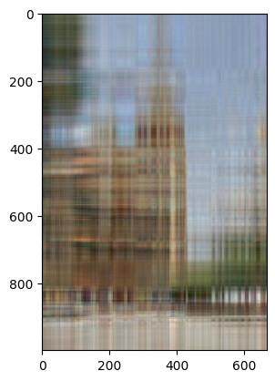
Recuerda que una imagen no es más que un conjunto de 3 matrices, cada una representando la intensidad de la grilla de píxeles para cada color (rojo, verde y azul). Una forma de comprimir una imagen consiste en quedarse con los \(k\) primeros valores singulares para cada color e intercambiar \(k\) por una se las dimensiones que representan el alto o el ancho de la imagen.
Crea una función aproxima_img que tome un array de dimensión \((3, h, w)\) y devuelva otra imagen aproximada de dimensión \((3, h, w)\) utilizando los k primeros valores singulares. Para ello,
Utiliza la función
scipy.misc.facepara generar una imagen de prueba, o también puedes importar una utilizandoim = cv2.imread("img.jpg"). Puedes visualizar imágenes con este formato a través del la funciónimshowdematplotlib.pyplot(a veces hay que cambiar de orden los canales).Utiliza la función
svddenp.linalgpara realizar la descomposición SVD. Mucho cuidado con las dimensiones que espera la función.Otras funciones que pueden ser útiles para el ejercicio:
np.transpose,np.zeros,np.fill_diagonal,np.clip.
import scipy
import matplotlib.pyplot as plt
import cv2
im = scipy.misc.face()
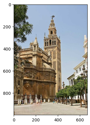
im_giralda = cv2.imread("giralda.jpg")
<ipython-input-27-658b7694cb54>:5: DeprecationWarning: scipy.misc.face has been deprecated in SciPy v1.10.0; and will be completely removed in SciPy v1.12.0. Dataset methods have moved into the scipy.datasets module. Use scipy.datasets.face instead.
  im = scipy.misc.face()
plt.imshow(im_giralda[:, :, [2, 1, 0]])
<matplotlib.image.AxesImage at 0x7a711ce634c0>
h, w, _ = im_giralda.shape
h, w
(1000, 667)
from numpy.linalg import svd

im_giralda_modificada = np.transpose(im_giralda, (2, 0, 1))
U, s, Vh = svd(im_giralda_modificada)
k = 5
S = np.zeros((3, w, w))
for c in range(3):
    np.fill_diagonal(S[c], s[c])
im_comprimida = U[:, :, :k] @ S[:, :k, :] @ Vh
im_comprimida = (im_comprimida - im_comprimida.min()) / (im_comprimida.max() - im_comprimida.min())
im_final = np.transpose(im_comprimida, (1, 2, 0))[:, :, [2, 1, 0]]
plt.imshow(im_final)
<matplotlib.image.AxesImage at 0x7a7109c7a080>
Exercise 57
Importa una imagen de tu elección utilizando la función imread de la librería cv2. Crea un array kernel de dimensión \((n, n)\) y realiza la convolución de tu imagen con kernel mediante la función scipy.signal.convolve2d (parámetro mode='same'). Si tu imagen tiene varios canales para los colores, aplica el mismo kernel a cada canal.
Algunos ejemplos interesantes de kernel pueden ser los siguientes:
\(n = 3\) con valores
transpuesta del anterior,
\(n \approx 50\), generados con
scipy.signal.windows.gaussian(puedes utilizar la funciónnp.outerpara realizar un producto exterior)Operador complejo de Sharr
scharr = np.array([[ -3-3j, 0-10j,  +3 -3j],

                   [-10+0j, 0+ 0j, +10 +0j],

                   [ -3+3j, 0+10j,  +3 +3j]])
Puedes visualizar las imágenes con matplotlib.pyplot.imshow.
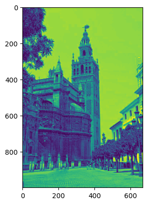
giralda = im_giralda[:, :, 0]
plt.imshow(giralda)
giralda.shape
(1000, 667)
im_giralda.shape
(1000, 667, 3)
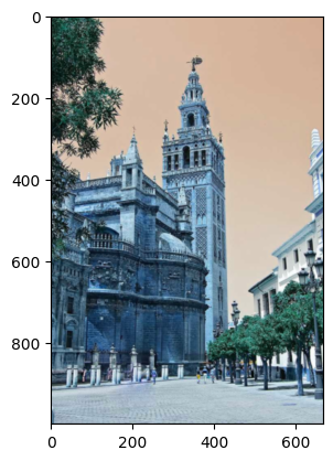
n = 20
v = scipy.signal.windows.gaussian(n, 1)
kernel = np.outer(v, v)
print(v)
[2.52616378e-20 2.04697171e-16 6.10193668e-13 6.69158609e-10
 2.69957850e-07 4.00652974e-05 2.18749112e-03 4.39369336e-02
 3.24652467e-01 8.82496903e-01 8.82496903e-01 3.24652467e-01
 4.39369336e-02 2.18749112e-03 4.00652974e-05 2.69957850e-07
 6.69158609e-10 6.10193668e-13 2.04697171e-16 2.52616378e-20]
import scipy
ret = np.zeros(im_giralda.shape)
for i in range(3):
    ret[:, :, i] = scipy.signal.convolve2d(
        im_giralda[:, :, i], kernel.T,
        mode="same"
    )
print(ret.shape)
(1000, 667, 3)
ret = (ret - ret.min()) / (ret.max() - ret.min())
plt.imshow(ret)
<matplotlib.image.AxesImage at 0x7a7109758790>
Regresión Lineal#
Exercise 58
Considera un modelo de regresión lineal que consiste en estimar una variable \(y\) como una suma ponderada de un cojunto de variables regresoras
donde
\(n\) es el conjunto de variables regresoras o features, \(x_i\) el valor correspondiente.
\(\hat{y}\) es el valor predicho.
\(\theta_i\) son parámetros del modelo para \(0 \leq i \leq n\).
Podemos expresar dicha ecuación en formato matricial como
Dado un conjunto de \(m\) observaciones, nuestro objetivo es encontrar \(\boldsymbol{\theta}\) tal que se minimice nuestra aproximación lineal en términos de menores cuadrados
El valor óptimo de los parámetros se puede calcular directamente
donde
es el conjunto de observaciones de las variables regresoras e
es el conjunto de observaciones de la variable objetivo.
Crea una clase RegresionLineal con dos métodos,
entrena: toma como parámetrosXey, observaciones de las variables regresoras y objetivo, respectivamente, y calcula los coeficientes de la regresión lineal y los guarda en un atributo_theta.transforma: toma como parámetro una serie de observaciones nuevasXy devuelve una estimacióny_hatde la varible objetivo utilizando el método descrito anteriormente.
Funciones que puede ser de ayuda: np.linalg.inv, np.linalg.pinv, np.vstack, np.hstack.
import numpy as np

a = np.array([1, 2, 3])
b = np.array([4, 5, 6])
ret = np.vstack((a, b, a))
np.vstack((ret, a))
array([[1, 2, 3],
       [4, 5, 6],
       [1, 2, 3],
       [1, 2, 3]])
a = np.array([1, 2, 3])
b = np.array([4, 5, 6])
ret = np.hstack((a, b, a))
np.hstack((ret, a))
array([1, 2, 3, 4, 5, 6, 1, 2, 3, 1, 2, 3])
class RegresionLineal:
    def entrena(self, X: np.ndarray, y: np.ndarray):
        self._theta = np.linalg.inv(X.T @ X) @ X.T @ y

    def transforma(self, X: np.ndarray):
        y_hat = X @ self._theta
        return y_hat
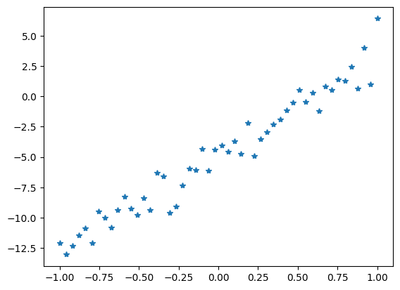
n = 20
m = 500
X = np.linspace(-1, 1, m)
y = -5 + 8*X + np.random.randn(m)
X = X.reshape((m, n))
X = np.hstack((np.ones(m).reshape(m, 1), X))
print(X.shape)
print(y.shape)
(50, 2)
(50,)
y
array([-12.07138479, -13.05330976, -12.30973441, -11.46320839,
       -10.88177573, -12.09517009,  -9.49463607, -10.02115952,
       -10.81179953,  -9.38041474,  -8.28437883,  -9.28292337,
        -9.77973295,  -8.41466714,  -9.39253765,  -6.30435892,
        -6.56187333,  -9.62431838,  -9.08033994,  -7.32173858,
        -5.98043991,  -6.08453968,  -4.33927567,  -6.14008111,
        -4.36088648,  -4.03233517,  -4.54459737,  -3.69984803,
        -4.75900016,  -2.15688479,  -4.9113157 ,  -3.49536467,
        -2.95591481,  -2.31966105,  -1.91955907,  -1.12208564,
        -0.50058478,   0.56198314,  -0.46281322,   0.33134371,
        -1.20940969,   0.81700321,   0.51475479,   1.43280438,
         1.27921539,   2.46556578,   0.65738281,   3.98946003,
         1.02193463,   6.42544706])
import matplotlib.pyplot as plt

plt.plot(X[:, 1], y, "*")
[<matplotlib.lines.Line2D at 0x7a71094eded0>]
regresion_lineal = RegresionLineal()

regresion_lineal.entrena(X, y)
regresion_lineal._theta
array([-4.82254328, 8.01213967])
regresion_lineal.transforma(X)
array([-12.83468295, -12.50765684, -12.18063074, -11.85360463,
       -11.52657852, -11.19955241, -10.8725263 , -10.54550019,
       -10.21847408,  -9.89144797,  -9.56442186,  -9.23739575,
        -8.91036965,  -8.58334354,  -8.25631743,  -7.92929132,
        -7.60226521,  -7.2752391 ,  -6.94821299,  -6.62118688,
        -6.29416077,  -5.96713467,  -5.64010856,  -5.31308245,
        -4.98605634,  -4.65903023,  -4.33200412,  -4.00497801,
        -3.6779519 ,  -3.35092579,  -3.02389969,  -2.69687358,
        -2.36984747,  -2.04282136,  -1.71579525,  -1.38876914,
        -1.06174303,  -0.73471692,  -0.40769081,  -0.0806647 ,
         0.2463614 ,   0.57338751,   0.90041362,   1.22743973,
         1.55446584,   1.88149195,   2.20851806,   2.53554417,
         2.86257028,   3.18959638])